Show code
library(psych)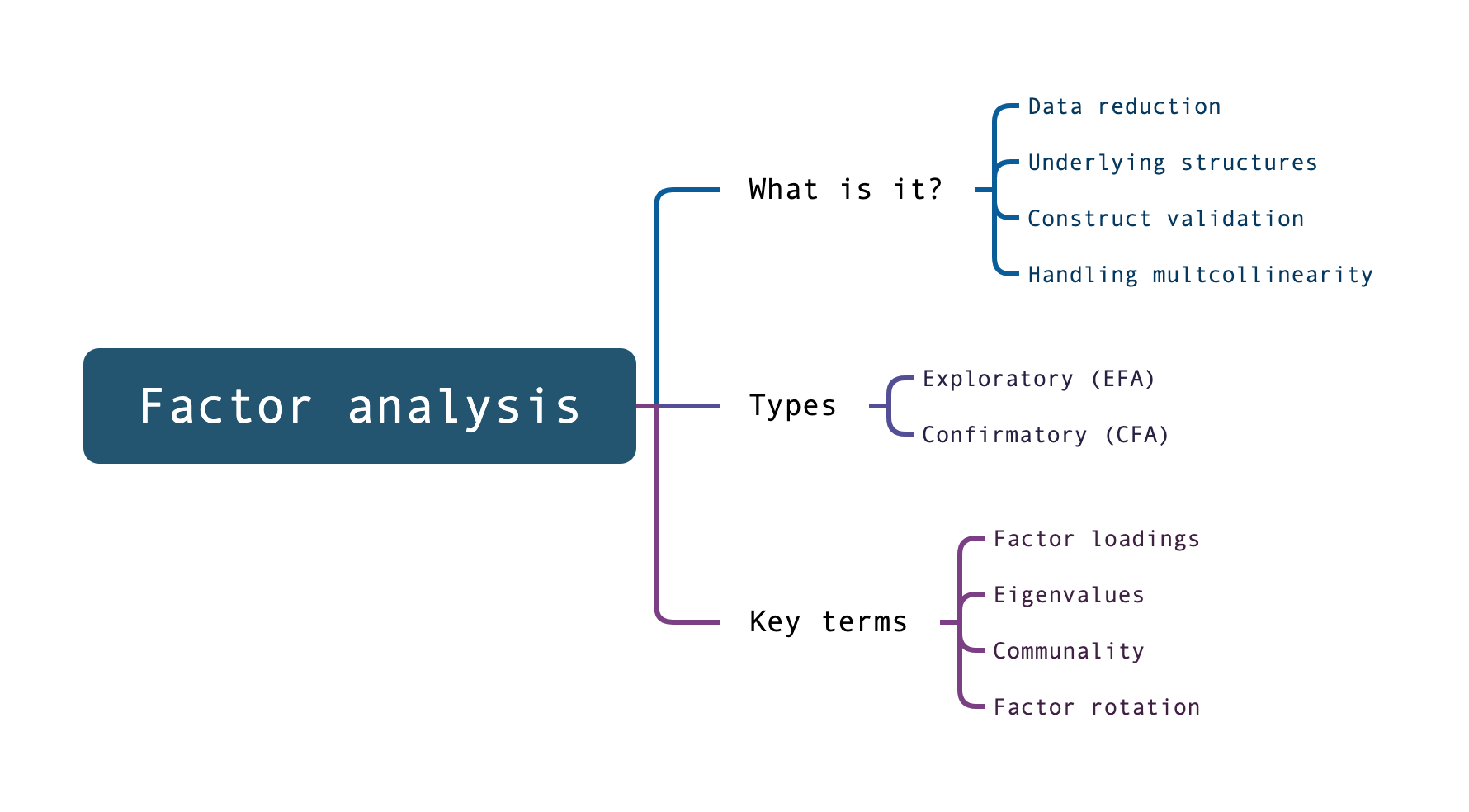
Before starting this practical, please make sure you have read the previous section.
In particular, make sure you understand some of the key terms such as ‘factor loadings’.
Factor analysis (FA) is a statistical procedure used to determine underlying factors within a set of variables.
It’s based on an assumption that there are underlying constructs/dimensions/factors that explain responses to different variables.
There are two types of factor analysis: exploratory factor analysis (EFA) and confirmatory factor analysis (CFA).
In this practical we’ll explore how to conduct both types of factor analysis in R. Please note that this is a substantial topic and this practical is designed to provide an introduction only to the subject.
Exploratory factor analysis is used to explore the possible underlying factor structure without imposing a preconceived structure on the outcome.
First, load the library psych which allows factor analysis to be conducted in R:
library(psych)Run the following code to download a dataset that we’ll work with:
efa_data <- read.csv('https://www.dropbox.com/scl/fi/e5qri07n3ng2jl3nxl47j/efa_data.csv?rlkey=qm6xyngabaz1iibxzuew57y0k&dl=1')

head(efa_data,6) # display the first six rows
x1 x2 x3 x4 x5 x6 x7 x8
1 41.81652 54.36609 48.59140 37.62583 43.26455 35.24287 44.03834 39.39594
2 46.38909 54.73417 40.92760 28.71853 25.30821 23.41793 34.04191 32.90530
3 65.47243 63.17818 61.76063 28.55799 30.74977 26.79952 43.06434 46.30937
4 53.21858 55.85951 52.32586 17.04806 24.24856 21.12678 33.36992 36.25736
5 54.46779 49.56945 57.20893 37.74145 34.39522 26.92147 49.60866 40.12148
6 67.78961 63.53888 57.58055 28.82692 32.73377 31.68236 47.60180 52.36406
x9
1 42.73451
2 38.62343
3 43.98453
4 32.86608
5 39.98561
6 46.68363The dataset contains nine variables, x1…x9.
In our analysis, we are going to explore whether there are some underlying factors that explain the responses we see to the individual variables.
Remember, factor analysis is based on the understanding that there are certain constructs that we can’t directly observe (like ‘fitness’) that underpin how people respond to different measurements of that construct (like ‘aerobic capacity’, ‘sprint time’ etc.)
As this is an exploratory analysis, we do not assume a certain number of factors or dimensions in our data. We want to explore this aspect of our data.
To do so, we run a parallel analysis to help decide how many factors to extract:
fa.parallel(efa_data, fa="both")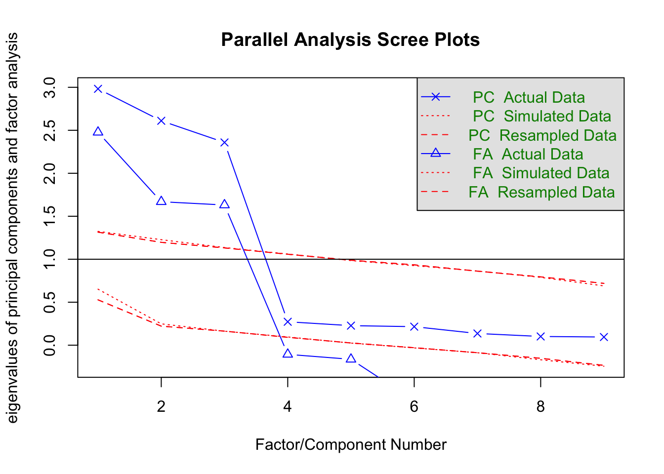
Parallel analysis suggests that the number of factors = 3 and the number of components = 3 Explanation
We’ve conducted a parallel analysis, a technique to determine the number of factors to retain in the factor analysis.
Remember, we’re starting off with no assumptions about how many factors may underpin our data.
By specifying fa="both", we are specifying the types of factor analysis to simulate when generating random data for comparison. The value “both” means that both principal axis factoring (fa=“pa”) and principal components analysis (fa=“pc”) will be used. In parallel analysis, eigenvalues from the actual data are compared against those derived from randomly generated data using these methods.
You may wish to explore these different methods (Principal Axis Factoring, Principal Components Analysis) in more detail.
The output of fa.parallel is usually a scree plot along with eigenvalues for both the actual data and the simulated data.
The number of factors to retain is suggested by the point where the actual data’s eigenvalues (PC/FA Actual Data) fall below the eigenvalues of the simulated data (PC/FA Simulated Data).
You’ll note also that our analysis helpfully prints the suggestion that there are three factors that ‘explain’ our data.
fa() function, specifying the number of factors (3) and rotation method (‘varimax’):efa_result <- fa(efa_data, nfactors=3, rotate="varimax")In this code:
efa_result is the variable where the results of the factor analysis will be stored. After running this line of code, efa_result will contain various outputs from the factor analysis, including factor loadings, uniquenesses, and the factor correlation matrix.
fa() is the function from the psych package that performs factor analysis. The fa() function is versatile and can be used for different types of factor analysis techniques.
nfactors=3 specifies the number of factors to extract from the data. In this case, it’s set to 3, meaning the function will identify and compute three underlying factors that explain the variance and correlations among the observed variables.
rotate="varimax" specifies the rotation method to be used in the factor analysis. Rotation methods are used to make the output of factor analysis more interpretable. “Varimax” is a type of orthogonal rotation that maximizes the variance of the squared loadings of a factor on all the variables.
In factor analysis, rotation methods are used to simplify and interpret the loadings of variables on factors. These methods can be broadly classified into two categories: orthogonal and oblique rotations.
Orthogonal Rotation:
Varimax Rotationis the most common method, and maximises the variance of the squared loadings of a factor. This method simplifies the interpretation by making factors as distinct as possible.
Quartimax Rotation aims to simplify the interpretation of variables, by minimising the number of factors needed to explain each variable.
Equamax Rotation is a hybrid of Varimax and Quartimax, seeking a balance between simplifying factors and simplifying variables.
Oblique Rotation:
Direct Oblimin Rotation allows factors to be correlated, providing a more realistic representation when factors are expected to be related.
Promax Rotation is an extension of Varimax, applied after an initial Varimax rotation. It allows for correlated factors and is computationally efficient, especially useful for large datasets.
Finally, we can inspect factor loadings and communalities. We’ll produce a visual map of our factors and their loadings on the different variables.
print(efa_result, cut=0.3) # Only show loadings greater than 0.3Factor Analysis using method = minres
Call: fa(r = efa_data, nfactors = 3, rotate = "varimax")
Standardized loadings (pattern matrix) based upon correlation matrix
MR1 MR2 MR3 h2 u2 com
x1 1.00 0.99 0.0066 1
x2 0.86 0.74 0.2624 1
x3 0.87 0.75 0.2487 1
x4 0.99 0.98 0.0209 1
x5 0.88 0.77 0.2316 1
x6 0.86 0.75 0.2455 1
x7 0.95 0.90 0.0994 1
x8 0.89 0.80 0.2010 1
x9 0.88 0.78 0.2240 1
MR1 MR2 MR3
SS loadings 2.50 2.48 2.48
Proportion Var 0.28 0.28 0.28
Cumulative Var 0.28 0.55 0.83
Proportion Explained 0.34 0.33 0.33
Cumulative Proportion 0.34 0.67 1.00
Mean item complexity = 1
Test of the hypothesis that 3 factors are sufficient.
df null model = 36 with the objective function = 8.04 with Chi Square = 1568.39
df of the model are 12 and the objective function was 0.05
The root mean square of the residuals (RMSR) is 0.01
The df corrected root mean square of the residuals is 0.01
The harmonic n.obs is 200 with the empirical chi square 0.58 with prob < 1
The total n.obs was 200 with Likelihood Chi Square = 9.06 with prob < 0.7
Tucker Lewis Index of factoring reliability = 1.006
RMSEA index = 0 and the 90 % confidence intervals are 0 0.056
BIC = -54.52
Fit based upon off diagonal values = 1
Measures of factor score adequacy
MR1 MR2 MR3
Correlation of (regression) scores with factors 0.99 1.00 0.97
Multiple R square of scores with factors 0.98 0.99 0.94
Minimum correlation of possible factor scores 0.96 0.99 0.89fa.diagram(efa_result)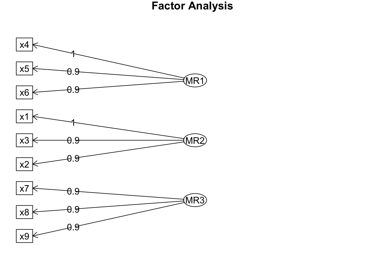
This final output shows us which of the variables loads most heavily on each of the three factors. For example, x1, x2 and x3 load most heavily on Factor 2.
This means that responses to each group of variables (e.g. x1, x2 and x3) are not independent, but may be explained by an underlying factor.
When we have identified the factors, there are a few different things we can do with them. For example:
Based on the items that load highly on each factor, we can interpret and name the factors. This involves understanding the underlying concept or construct that each factor represents.
The naming should be reflective of the common theme or characteristic shared by the variables with high loadings on that factor.
# show the factor loadings for existing variables
print(efa_result$loadings)
Loadings:
   MR1    MR2    MR3
x1         0.995
x2         0.859
x3         0.866
x4  0.989
x5  0.875
x6  0.864
x7                0.948
x8                0.893
x9                0.877

                 MR1   MR2   MR3
SS loadings    2.501 2.481 2.478
Proportion Var 0.278 0.276 0.275
Cumulative Var 0.278 0.554 0.829# calculate factor scores
factor_scores <- efa_result[["scores"]]Now, we can use these factor variables instead of our original variables for subsequent analysis (e.g., regression).
# Combine original data with factor scores
combined_efa_data <- cbind(efa_data, factor_scores)

head(combined_efa_data)
x1 x2 x3 x4 x5 x6 x7 x8
1 41.81652 54.36609 48.59140 37.62583 43.26455 35.24287 44.03834 39.39594
2 46.38909 54.73417 40.92760 28.71853 25.30821 23.41793 34.04191 32.90530
3 65.47243 63.17818 61.76063 28.55799 30.74977 26.79952 43.06434 46.30937
4 53.21858 55.85951 52.32586 17.04806 24.24856 21.12678 33.36992 36.25736
5 54.46779 49.56945 57.20893 37.74145 34.39522 26.92147 49.60866 40.12148
6 67.78961 63.53888 57.58055 28.82692 32.73377 31.68236 47.60180 52.36406
x9 MR1 MR2 MR3
1 42.73451 0.92381100 -0.8029808 0.3351331
2 38.62343 -0.19281286 -0.4541587 -0.7369188
3 43.98453 -0.14973554 1.6413984 0.6444454
4 32.86608 -1.40414619 0.2940866 -0.7452817
5 39.98561 0.80702695 0.4969310 0.7321430
6 46.68363 -0.08179012 1.9216559 1.2989276Note: do not delete efa_data…we’ll need it later in the practical.
Step One: Create a dataframe df by running the following code:
df <- read.csv('https://www.dropbox.com/scl/fi/u3d9l1ffka4mdzoa7xrfo/efa.csv?rlkey=gw7wxakp8hvvd6s95k9f5q01h&dl=1')Step Two: Now, using the psych package, determine the number of factors in the data using a scree plot. Check back to review how the information in the scree plot helps us determine the appropriate number of factors to extract.
library(psych)
fa.parallel(df, fa="both")

# your plot should show that there are three factors within the data.
Step Three: Based on the output of that analysis, conduct a factor analysis using the fa command. Insert the correct number of factors in your code, and choose varimax as the rotation option.
df_result <- fa(df, nfactors=3, rotate="varimax")Step Four: Inspect that solution. Include a visual representation of your analysis.
print(df_result, cut=0.3)  # Only show loadings greater than 0.3
fa.diagram(df_result)
How would you interpret this analysis? What does it suggest about underlying factors in the data?
Step Five: Integrate the factor loadings into a new dataset called combined_df.
# Combine original data with factor scores
combined_df_data <- cbind(df, factor_scores)

head(combined_df_data)We are now going to conduct a CFA on the dataset efa_data, which should be in your Environment.
In our EFA demonstration, we did not start with any assumptions about the number of factors in our dataset.
EFA is most appropriate in those situations.
However, there will be situations where we do have an idea about how many factors/dimensions might underpin our data, and we simply want to test this idea.
This is where confirmatory factor analysis is useful. It is used to ‘confirm’ our assumptions or hypotheses.
library(lavaan) # this library is recommended for CFARemember that CFA is based on a prior prediction of the factors that underpin our model. We might define our model based on previous EFA results, or theoretical assumptions (based on our knowledge of field, for example).
CFA can also be used to confirm the results produced by EFA. In this practical, we are going to continue to CFA with the previous dataset efa_data.
We’re going to test the possibility that there are three factors underlying our data, and that certain variables load most heavily on each factor.
Note that we have good reason to suspect this will be the case, because our EFA suggest it’s true.
The syntax in lavaan is straightforward.
For example, to conduct a CFA for a model with three factors (F1, F2 and F3) and nine variables (x1…x9) we can propose the following, based on the results of our EFA:
model <- '
  F1 =~ x4 + x5 + x6
  F2 =~ x1 + x2 + x3
  F3 =~ x7 + x8 + x9
'
Here, x1 to x9 are the observed variables, and =~ indicates which variables are indicators of which factors (F1 to F3).
In simple terms, we’re looking to confirm if the variables (x1…x9) that we think are explained by each factor do, in fact, conform to this prediction.
In the current analysis, we have based our allocation of variables to factors on the results from our EFA above.
Sometimes, you might be dealing with a questionnaire or other measure where you think that certain responses (variables) reflect an underlying factor.
We run the CFA process on the model we just created:
# Run the CFA
fit <- cfa(model, data=efa_data)
This produces an object called fit, which contains all the information about the model. You’ll see it in the Environment window.
Visual presentations can help us understand our model. The following code provides a useful way to produce such a visualisation.
You’ll need the semPlot package installed for this.
library(semPlot)

# a path diagram
semPaths(fit, whatLabels = "est", layout = "tree", edge.label.cex = 0.8,
         nCharNodes = 0, nCharEdges = 0, sizeMan = 10, sizeLat = 10)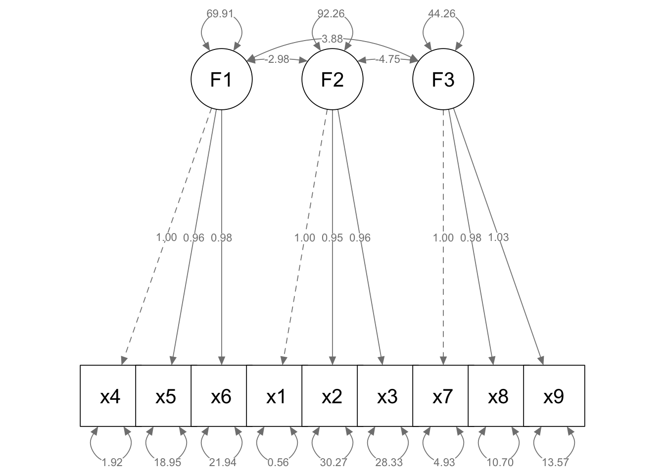
What does this plot tell us? It shows us which variables load most heavily on each of the factors (F1 etc.).
In this model F1 is the same as MR1 in our previous CFA analysis.
We can now check various fit indices to see if our model is a ‘good’ one or not.
# Summarize the results
summary(fit, fit.measures=TRUE)
lavaan 0.6.17 ended normally after 137 iterations
Estimator ML
Optimization method NLMINB
Number of model parameters 21
Number of observations 200
Model Test User Model:
Test statistic 18.578
Degrees of freedom 24
P-value (Chi-square) 0.774
Model Test Baseline Model:
Test statistic 1607.229
Degrees of freedom 36
P-value 0.000
User Model versus Baseline Model:
Comparative Fit Index (CFI) 1.000
Tucker-Lewis Index (TLI) 1.005
Loglikelihood and Information Criteria:
Loglikelihood user model (H0) -5674.233
Loglikelihood unrestricted model (H1) -5664.944
Akaike (AIC) 11390.465
Bayesian (BIC) 11459.730
Sample-size adjusted Bayesian (SABIC) 11393.200
Root Mean Square Error of Approximation:
RMSEA 0.000
90 Percent confidence interval - lower 0.000
90 Percent confidence interval - upper 0.040
P-value H_0: RMSEA <= 0.050 0.981
P-value H_0: RMSEA >= 0.080 0.000
Standardized Root Mean Square Residual:
SRMR 0.026
Parameter Estimates:
Standard errors Standard
Information Expected
Information saturated (h1) model Structured
Latent Variables:
Estimate Std.Err z-value P(>|z|)
F1 =~
x4 1.000
x5 0.956 0.044 21.567 0.000
x6 0.977 0.047 20.812 0.000
F2 =~
x1 1.000
x2 0.954 0.047 20.241 0.000
x3 0.960 0.046 20.823 0.000
F3 =~
x7 1.000
x8 0.979 0.047 20.653 0.000
x9 1.028 0.052 19.948 0.000
Covariances:
Estimate Std.Err z-value P(>|z|)
F1 ~~
F2 -2.976 5.766 -0.516 0.606
F3 3.880 4.109 0.944 0.345
F2 ~~
F3 -4.751 4.681 -1.015 0.310
Variances:
Estimate Std.Err z-value P(>|z|)
.x4 1.923 1.682 1.143 0.253
.x5 18.947 2.435 7.782 0.000
.x6 21.941 2.713 8.088 0.000
.x1 0.562 2.297 0.245 0.807
.x2 30.275 3.679 8.229 0.000
.x3 28.330 3.535 8.013 0.000
.x7 4.934 1.244 3.965 0.000
.x8 10.703 1.532 6.988 0.000
.x9 13.571 1.817 7.470 0.000
F1 69.906 7.372 9.482 0.000
F2 92.263 9.562 9.649 0.000
F3 44.264 5.027 8.806 0.000# Alternatively, you can use standardised results
summary(fit, fit.measures=TRUE, standardized=TRUE)lavaan 0.6.17 ended normally after 137 iterations
Estimator ML
Optimization method NLMINB
Number of model parameters 21
Number of observations 200
Model Test User Model:
Test statistic 18.578
Degrees of freedom 24
P-value (Chi-square) 0.774
Model Test Baseline Model:
Test statistic 1607.229
Degrees of freedom 36
P-value 0.000
User Model versus Baseline Model:
Comparative Fit Index (CFI) 1.000
Tucker-Lewis Index (TLI) 1.005
Loglikelihood and Information Criteria:
Loglikelihood user model (H0) -5674.233
Loglikelihood unrestricted model (H1) -5664.944
Akaike (AIC) 11390.465
Bayesian (BIC) 11459.730
Sample-size adjusted Bayesian (SABIC) 11393.200
Root Mean Square Error of Approximation:
RMSEA 0.000
90 Percent confidence interval - lower 0.000
90 Percent confidence interval - upper 0.040
P-value H_0: RMSEA <= 0.050 0.981
P-value H_0: RMSEA >= 0.080 0.000
Standardized Root Mean Square Residual:
SRMR 0.026
Parameter Estimates:
Standard errors Standard
Information Expected
Information saturated (h1) model Structured
Latent Variables:
Estimate Std.Err z-value P(>|z|) Std.lv Std.all
F1 =~
x4 1.000 8.361 0.987
x5 0.956 0.044 21.567 0.000 7.997 0.878
x6 0.977 0.047 20.812 0.000 8.167 0.867
F2 =~
x1 1.000 9.605 0.997
x2 0.954 0.047 20.241 0.000 9.165 0.857
x3 0.960 0.046 20.823 0.000 9.219 0.866
F3 =~
x7 1.000 6.653 0.949
x8 0.979 0.047 20.653 0.000 6.514 0.894
x9 1.028 0.052 19.948 0.000 6.839 0.880
Covariances:
Estimate Std.Err z-value P(>|z|) Std.lv Std.all
F1 ~~
F2 -2.976 5.766 -0.516 0.606 -0.037 -0.037
F3 3.880 4.109 0.944 0.345 0.070 0.070
F2 ~~
F3 -4.751 4.681 -1.015 0.310 -0.074 -0.074
Variances:
Estimate Std.Err z-value P(>|z|) Std.lv Std.all
.x4 1.923 1.682 1.143 0.253 1.923 0.027
.x5 18.947 2.435 7.782 0.000 18.947 0.229
.x6 21.941 2.713 8.088 0.000 21.941 0.248
.x1 0.562 2.297 0.245 0.807 0.562 0.006
.x2 30.275 3.679 8.229 0.000 30.275 0.265
.x3 28.330 3.535 8.013 0.000 28.330 0.250
.x7 4.934 1.244 3.965 0.000 4.934 0.100
.x8 10.703 1.532 6.988 0.000 10.703 0.201
.x9 13.571 1.817 7.470 0.000 13.571 0.225
F1 69.906 7.372 9.482 0.000 1.000 1.000
F2 92.263 9.562 9.649 0.000 1.000 1.000
F3 44.264 5.027 8.806 0.000 1.000 1.000This looks complex (and it is!).
To keep things simple, for now, look for CFI and TLI values close to or above 0.95, and RMSEA values below 0.06 for a good fit.
Results like this will confirm that the model we provided (the three factors, and each variable loading onto one of them) is a good ‘fit’ (or ‘explanation’) for the variance we observe within our individual variables.
If we have different proposed models (for example, we might wonder if there are actually only two underlying factors), we can re-run the model and compare the output of these tests to see which model is ‘better’ in terms of overall fit.
Repeat all of these steps on the dataset df, which you used for the EFA practice.
You should: load the lavaan library; specify your model; fit the model; visually inspect your model; check model fit.
Remember, the result of that analysis was that there were three underlying factors, and you identified which variables loaded most heavily on each of those factors.
#---------------------------
# Step One: Load library
#---------------------------

library(lavaan) # this library is recommended for CFA

#---------------------------
# Step Two: Specify model
#---------------------------

model <- '
  F2 =~ Var1 + Var6 + Var3 + Var10 + Var2
  F1 =~ Var5 + Var7 + Var9
  F3 =~ Var4 + Var8
'
#---------------------------
# Step Three: Fit the model
#---------------------------

# Run the CFA
cfa_fit <- cfa(model, data=df)

#---------------------------
# Step Four: Visual inspection of the model
#---------------------------

library(semPlot)

# a path diagram
semPaths(cfa_fit, whatLabels = "est", layout = "tree", edge.label.cex = 0.8,
         nCharNodes = 0, nCharEdges = 0, sizeMan = 10, sizeLat = 10)

#---------------------------
# Step Five: Assess model fit
#---------------------------

# Summarize the results
summary(cfa_fit, fit.measures=TRUE)

# Alternatively, you can use standardised results
summary(cfa_fit, fit.measures=TRUE, standardized=TRUE)